noise2: A Weather Map of Smooth Randomness
Part 7 of 7 in our series of stdlib primers — the deterministic hash, noise, and shaping functions.
Series: Stdlib Primers
- hash01 — a random number that never changes its mind
- hash11 — the same dice, rolled between −1 and 1
- hashRange — randomRange with a memory
- smoothstep — the S-curve that turns a cliff into a ramp
- bump — a hill you can put anywhere
- noise — randomness with a smooth ride
- noise2 (this post) — a weather map of smooth randomness
What it does
noise wanders along a line. noise2(x, y, seed?)
spreads the same smooth randomness across a surface — fog, terrain,
water, or "many strokes that agree with their neighbors."
Extend the pins model to a pegboard: random heights pinned at every
whole-number grid corner. Anywhere inside a cell, the answer smoothly
mixes the four surrounding corner pins — nearer corners count more. That
one sentence is the whole mechanism. As with 1D noise, the mixing uses the
flat-arriving smoothstep glide, so the field
has no seams, and answers stay in [0, 1).
The second coordinate wears three costumes in practice:
- A real y — you're sampling an actual 2D field (fog, terrain).
- A layer index — line or layer
jsamples rowj * someScale, so siblings stay coherent: neighbors in the stack sample neighboring rows of one field. - A phase/time — slide
yslowly to animate a 1D wobble. (Worth knowing about; not built in these examples.)
One honesty note: this is the simple corner-value kind of noise, not the fancier "Perlin" kind that stores slopes at the pins. At large scales you can spot faint row-and-column grain in it; at the scales in this post, you won't.
Why you'd use it
Whenever smooth randomness needs to vary in two directions at once — across a grid of cells, over the area of a texture, or across a family of related strokes. That last one is the sleeper use: give each stroke in a stack its own row of one shared field and the whole stack starts behaving like a single surface. It's the difference between sixteen strokes that shimmer independently and one glow that flows.
Example 1 — Fog on a grid
The 2D field made visible, against its opposite. Both panels shade a
16×16 grid from the same palette; the left asks hash01 of each cell's
index, the right asks noise2 of each cell's position.
//-- Two shaded grids, same size, same palette. Left: each cell's shade is
//-- hash01 of its index -- TV static. Right: noise2 of its (col, row)
//-- position scaled down -- cloudy patches. Neighboring cells agree in
//-- BOTH directions.

define ViewBox(0, 0, 400, 220);

//-- Shades are bucketed into 16 layers per panel (not one per cell) to
//-- keep the SVG lean -- fine enough that the stepping doesn't read as
//-- banding.
fn panel(prefix, x0, useNoise) {
  for (b in 0..15) {
    let L = 0.28 + b * 0.0325;
    let c = Color(L, 0.04, 265);
    let bucketLayer = PathLayer(`${prefix}-b${b}`) #{ fill: c; stroke: none; };
    bucketLayer.apply {
      for (row in 0..15) {
        for (col in 0..15) {
          let v = 0;
          if (useNoise == 1) {
            v = noise2(col * 0.22, row * 0.22);
          }
          if (useNoise == 0) {
            v = hash01(row * 16 + col);
          }
          if (floor(v * 16) == b) {
            rect(calc(x0 + col * 10.3), calc(40 + row * 10.3), 9.8, 9.8);
          }
        }
      }
    }
  }
}

panel('static', 22, 0);
panel('fog', 208, 1);

let labels = TextLayer('labels') #{
  font-family: system-ui, sans-serif;
  font-size: 10;
  fill: #888;
  text-anchor: start;
};
labels.apply {
  text(22, 28)`hash01(idx) — static`
  text(208, 28)`noise2(col·0.22, row·0.22) — fog`
}
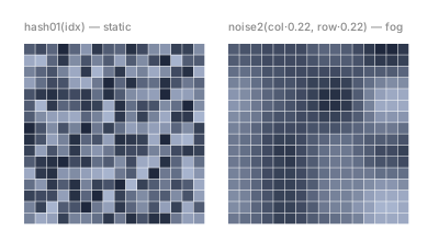
Static versus weather. In the right panel, every cell agrees with its neighbors up, down, left, and right — that's the "nearer corners count more" mixing at work. (Implementation note: the shades are bucketed into sixteen layers instead of one layer per cell — a useful economy whenever a grid gets large.)
Example 2 — Swelling dot field
Sampling the field at each element's own position. A 30×17 dot grid where
each radius is 0.6 + 3 * noise2(col * 0.12, row * 0.12).
//-- A 30 x 17 dot grid where each dot's radius samples the field at its
//-- own position: 0.6 + 3 * noise2(col * 0.12, row * 0.12). Sizes swell
//-- in blobs, like rain intensity across pavement.

define ViewBox(0, 0, 400, 220);

let dots = PathLayer('field') #{ fill: oklch(0.66 0.14 220); stroke: none; };
dots.apply {
  for (row in 0..16) {
    for (col in 0..29) {
      let v = noise2(col * 0.12, row * 0.12);
      circle(calc(26 + col * 12), calc(38 + row * 10.2), calc(0.6 + 3 * v));
    }
  }
}

let labels = TextLayer('labels') #{
  font-family: system-ui, sans-serif;
  font-size: 10;
  fill: #888;
  text-anchor: start;
};
labels.apply {
  text(26, 27)`radius = 0.6 + 3 · noise2(col·0.12, row·0.12)`
}
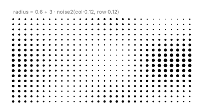
The sizes swell in blobs, like rain intensity across pavement. The
* 0.12 on both coordinates is the
frequency knob in 2D: smaller factors give bigger
weather systems, larger factors give choppier ones — tune it exactly as
you did in part 6.
Example 3 — Rows of one field
The layer-index costume, and the visual argument for this function's
existence. Left: line j samples noise2(t*4, j*0.3) — twelve rows of
one field, so neighboring lines rise and fall together and the stack
reads as a flowing sheet. Right: the same twelve lines with independent
1D streams — they ignore each other.
//-- The layer-index trick. Left stack: line j samples noise2(t*4, j*0.3)
//-- -- rows of ONE field, so neighboring lines rise and fall together and
//-- the stack reads as a flowing sheet. Right stack: each line gets its
//-- own independent 1D stream -- the lines ignore each other.

define ViewBox(0, 0, 400, 230);

fn strandCoherent(name, y0, j) {
  let line = PathLayer(name) #{ stroke: oklch(0.66 0.14 220); stroke-width: 1.3; fill: none; };
  line.apply {
    M 22 calc(y0 - noise2(0, j * 0.3) * 26)
    for (i in 1..56) {
      let t = i / 56;
      L calc(22 + t * 165) calc(y0 - noise2(t * 4, j * 0.3) * 26)
    }
  }
}

fn strandIndependent(name, y0, j) {
  let line = PathLayer(name) #{ stroke: oklch(0.62 0.1 300); stroke-width: 1.3; fill: none; };
  line.apply {
    M 213 calc(y0 - noise(0, j) * 26)
    for (i in 1..56) {
      let t = i / 56;
      L calc(213 + t * 165) calc(y0 - noise(t * 4, j) * 26)
    }
  }
}

for (j in 0..11) {
  let y = 62 + j * 13;
  strandCoherent(`sheet-${j}`, y, j);
  strandIndependent(`solo-${j}`, y, j);
}

let labels = TextLayer('labels') #{
  font-family: system-ui, sans-serif;
  font-size: 10;
  fill: #888;
  text-anchor: start;
};
labels.apply {
  text(22, 26)`noise2(t·4, j·0.3) — one field`
  text(213, 26)`noise(t·4, j) — independent seeds`
}
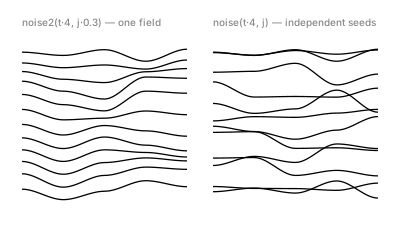
The only difference between the stacks is where the second number goes:
noise2(t*4, j*0.3) versus noise(t*4, j). As a coordinate, j puts
the lines on the same continuous surface; as a seed, it isolates them.
Choosing between those two spellings is choosing between coherence and
independence.
Example 4 — Warp a grid
Displacement: two fields make a push direction. Every vertex of a ruled
grid moves horizontally by field 0 and vertically by field 1 —
(noise2(x, y) - 0.5) * 14 each way (the - 0.5 recenters [0,1) into a
signed push, the same remap trick from hash11).
//-- Displacement: two fields make a push direction. Every vertex of a
//-- ruled grid moves by ((noise2(x,y) - 0.5) * 14, (noise2(x,y,1) - 0.5) * 14)
//-- -- the default field pushes horizontally, the seed-1 field vertically.
//-- The low frequency (0.14) keeps neighboring vertices agreeing, so the
//-- grid billows like a flag instead of crumpling.

define ViewBox(0, 0, 400, 230);

fn warpX(gx, gy) {
  return (noise2(gx * 0.14, gy * 0.14) - 0.5) * 14;
}
fn warpY(gx, gy) {
  return (noise2(gx * 0.14, gy * 0.14, 1) - 0.5) * 14;
}

let grid = PathLayer('warped-grid') #{ stroke: oklch(0.64 0.12 200); stroke-width: 1; fill: none; };
grid.apply {
  //-- Horizontal rules
  for (gy in 0..12) {
    let x0 = calc(30 + warpX(0, gy));
    let y0 = calc(28 + gy * 14.5 + warpY(0, gy));
    M x0 y0
    for (gx in 1..24) {
      let x = calc(30 + gx * 14.2 + warpX(gx, gy));
      let y = calc(28 + gy * 14.5 + warpY(gx, gy));
      L x y
    }
  }
  //-- Vertical rules
  for (gx in 0..24) {
    let x0 = calc(30 + gx * 14.2 + warpX(gx, 0));
    let y0 = calc(28 + warpY(gx, 0));
    M x0 y0
    for (gy in 1..12) {
      let x = calc(30 + gx * 14.2 + warpX(gx, gy));
      let y = calc(28 + gy * 14.5 + warpY(gx, gy));
      L x y
    }
  }
}
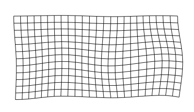
The grid billows like a flag because both displacement fields are smooth: neighboring vertices get nearly the same push, so the rules bend instead of scattering. Warping positions through a pair of fields like this is the doorway to flow fields, fabric, and water — all "move everything, but smoothly, and differently everywhere."
Example 5 — The flowing glow
The series finale, combining five posts. Twelve glow layers whose width
profile is bump algebra, each multiplied by a
texture factor 1 + (noise2(t*6, k*0.3) - 0.5) * 0.9 — with t running
along the stroke and layer index k running across the field.
//-- The series finale: bump-shaped widths (part 5) textured by ONE
//-- noise2 field. t runs along the stroke; layer * 0.3 runs across the
//-- layers. Because the field is continuous in both directions,
//-- neighboring layers sample neighboring rows -- and the whole glow
//-- flows as one surface instead of shimmering.

define ViewBox(0, 78, 400, 103);

let spine = @{ c 80 -100 160 100 240 0 };
let px = 80;
let py = 130;
let taperCap = Cap.tapered(2, CurveContinuity.G0);
let base = oklch(0.72 0.14 20);

for (k in 12..1) {
  let texture = {|t| return 1 + (noise2(t * 6, k * 0.3) - 0.5) * 0.9; };
  let mk = {|vo, pb|
    vo.startCap(taperCap);
    for (i in 0..47) {
      let t = i / 47;
      let w = (0.15 * k
            + 0.6 * k * bump(t, 0.35, 0.3)
            + 0.35 * k * pow(bump(t, 0.78, 0.18), 2)) * texture(t);
      vo.stop(t, w, CurveContinuity.G1, -w, CurveContinuity.G1);
    }
    vo.endCap(taperCap);
  };
  let halo = spine.compoundVariableOffset() << mk;

  let haloColor = base.hueShift(calc(k * -6));
  let haloLayer = PathLayer(`halo-${k}`) #{
    fill: haloColor;
    stroke: none;
    opacity: 0.25;
  };
  haloLayer.apply {
    M calc(px + halo.anchor.x) calc(py + halo.anchor.y)
    halo.draw();
  }
}
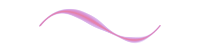
This series has now built the same glow three ways, and the differences
are the lesson. bump's finale is clean
architecture — smooth swells, nothing else.
hash11's ±wobble would make it shimmer, every
stop independent. This one makes it flow: watch the striations —
neighboring layers swell together as one surface, because everything
samples one continuous field. One argument's costume change (seed → row
coordinate) is the entire difference between shimmer and weather.
Where to go next
noise— the 1D story: pins, glide, frequency.bump— the width profiles under this finale's texture.hash01— the 1D pins. (noise2's corners hash both coordinates as a pair, so there's no directhash01equivalence in 2D — the exact-identity story is a 1D privilege.)- Reference: Hash & Noise docs — and that's the series. Seven functions, one promise: randomness, smoothness, and shape you can direct, tune, and ship.